जानें कि projection और reshuffle simulations आपकी Trade history को fan charts, Drawdown ranges और जांचे जा सकने वाले risk questions में कैसे बदलते हैं।
हम Tradeways को बेहतर बनाने के लिए analytics सहित cookies का उपयोग करते हैं। · गोपनीयता
आपकी historical इक्विटी कर्व results का एक क्रम दिखाती है: वह क्रम जो वास्तव में हुआ। Monte Carlo simulation पूछता है कि यही evidence कई alternative paths में कैसा दिख सकता था। यह Trades को बेहतर नहीं बनाता और market का अनुमान नहीं लगाता। यह दिखाता है कि पुराने outcomes का क्रम और दोहराव उस रास्ते को कितना बदल सकता है जिससे आपको Trade करना पड़ता।
इस फर्क के कारण simulation एक ठोस काम में उपयोगी है: यह जांचना कि strategy की दिखने वाली stability किसी एक अनुकूल क्रम पर निर्भर है या नहीं। Result conditional outcomes की range है, forecast नहीं।
Projection: अगर इस filtered sample जैसे results अगली Trades में दोहराएं, तो outcomes की range क्या हो सकती है?
Reshuffle: अगर यही Trades किसी दूसरे क्रम में आतीं, तो रास्ता कितना अलग हो सकता था?
दोनों modes समान source data इस्तेमाल करते हैं, लेकिन अलग सवालों के जवाब देते हैं। उन्हें एक जैसा मानना output को गलत पढ़ने का आसान तरीका है।
Tradeways आपके actual imported Trades से browser में दोनों modes चलाता है। Active account scope और live Trade filters input तय करते हैं। इसलिए win rate और payoff estimates दोबारा लिखे बिना strategy, सिंबल, दिशा, अवधि या दूसरे supported filter को अलग किया जा सकता है। Scope बदलने पर Monte Carlo analysis update होता है और result को पुराने Trades से बना simulation label करता है, forecast नहीं।
Projection mode filtered historical outcomes में से एक-एक Trade draw करके हर path बनाता है। किसी एक run में result एक से ज्यादा बार draw हो सकता है या बिल्कुल नहीं। इसे sampling with replacement कहते हैं।
आप horizon चुनते हैं, जैसे अगली 100 Trades, और simulation इस process को कई बार दोहराता है। Output दिखाता है कि एक साफ assumption के तहत paths और final outcomes कितने फैले हुए हैं: selected history उन outcomes के लिए उपयोगी model है जो आगे दोहरा सकते हैं।
Projection तब उपयुक्त है जब सवाल future को लेकर हो लेकिन शर्तों पर आधारित हो। यह दिखा सकता है कि positive historical average के बावजूद losing paths, गहरे Drawdown या लंबे recovery periods संभव हैं। यह नहीं बता सकता कि strategy का Edge बना रहेगा, market conditions बदलेंगी या future Trades उसी distribution का पालन करेंगी।
Reshuffle mode हर path में filtered sample की हर Trade को ठीक एक बार इस्तेमाल करता है और केवल उनका क्रम बदलता है। Additive P&L view में हर path इसलिए समान total पर खत्म होता है। उस total तक पहुंचने का रास्ता बदलता है: losing streaks, equity peaks, recovery timing और maximum Drawdown।
यह mode attribution का सवाल पूछता है। Historical curve smooth दिखती हो लेकिन कई alternative orders में काफी गहरे Drawdown हों, तो smoothness का कुछ हिस्सा अच्छे sequence से आया था। अलग orders में Drawdown distribution छोटा रहे, तो observed path wins और losses के समय पर कम निर्भर था।
Reshuffling नए Trade outcomes नहीं बनाता और अगली Trades का अनुमान नहीं लगाता। यह original sequence की serial structure भी तोड़ता है। अगर outcomes regimes, overlapping positions या sizing में जानबूझकर किए बदलावों पर निर्भर हैं, तो result को उन dependencies का model नहीं, ordering test मानें।
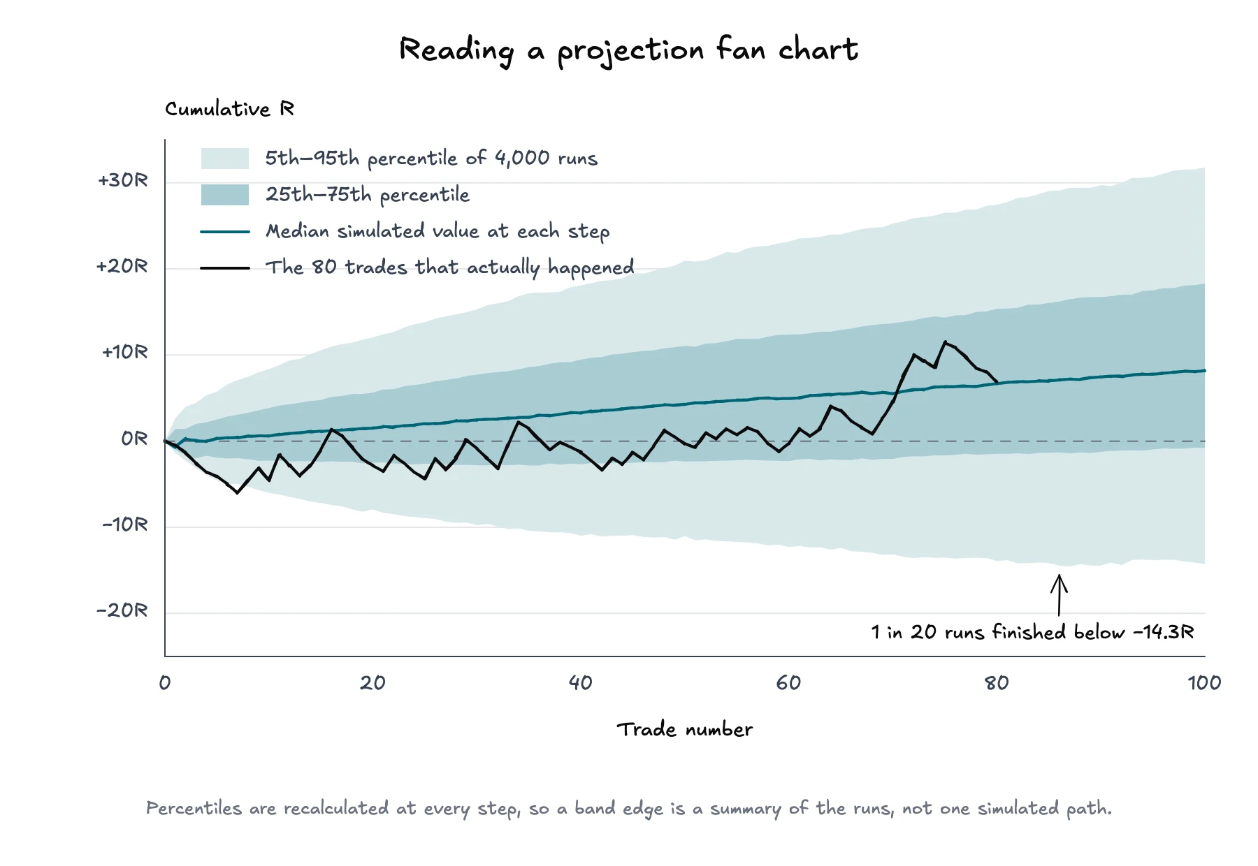
Fan chart horizontal axis पर Trade count और vertical axis पर cumulative outcome दिखाता है। हर step पर simulation सभी path values को sort करके percentiles mark करता है। Median line बीच का simulated value है। 5th से 95th percentile जैसी चौड़ी bands simulated dispersion का बड़ा हिस्सा दिखाती हैं।
एक उदाहरण projection: 80 filtered historical Trades से draw की गई 100 Trades के 4,000 runs। समान evidence से median बढ़ता है, लेकिन 5th percentile नहीं।
Chart को तीन steps में पढ़ें:
बीच देखें। Median हर Trade count पर बीच का simulated outcome दिखाता है। यह expected path या वादा नहीं है।
चौड़ाई देखें। तेजी से चौड़ा होता fan बताता है कि चुने assumptions के तहत sequence cumulative outcomes की बड़ी range बनाता है।
Actual curve की तुलना करें। Historical path दिखाता है कि realized sequence simulated range के मुकाबले कहां है। Outer band के पास path इस model में असामान्य है। इससे यह साबित नहीं होता कि हर संभव model में strategy या execution असामान्य थी।
Percentile boundaries हर step पर अलग calculate होती हैं। इसलिए 5th-percentile line जरूरी नहीं कि किसी एक continuous simulated path को दिखाए। इसका यह मतलब भी नहीं कि future equity के उससे ऊपर रहने की 95% संभावना है। यह runs का point-by-point summary है।
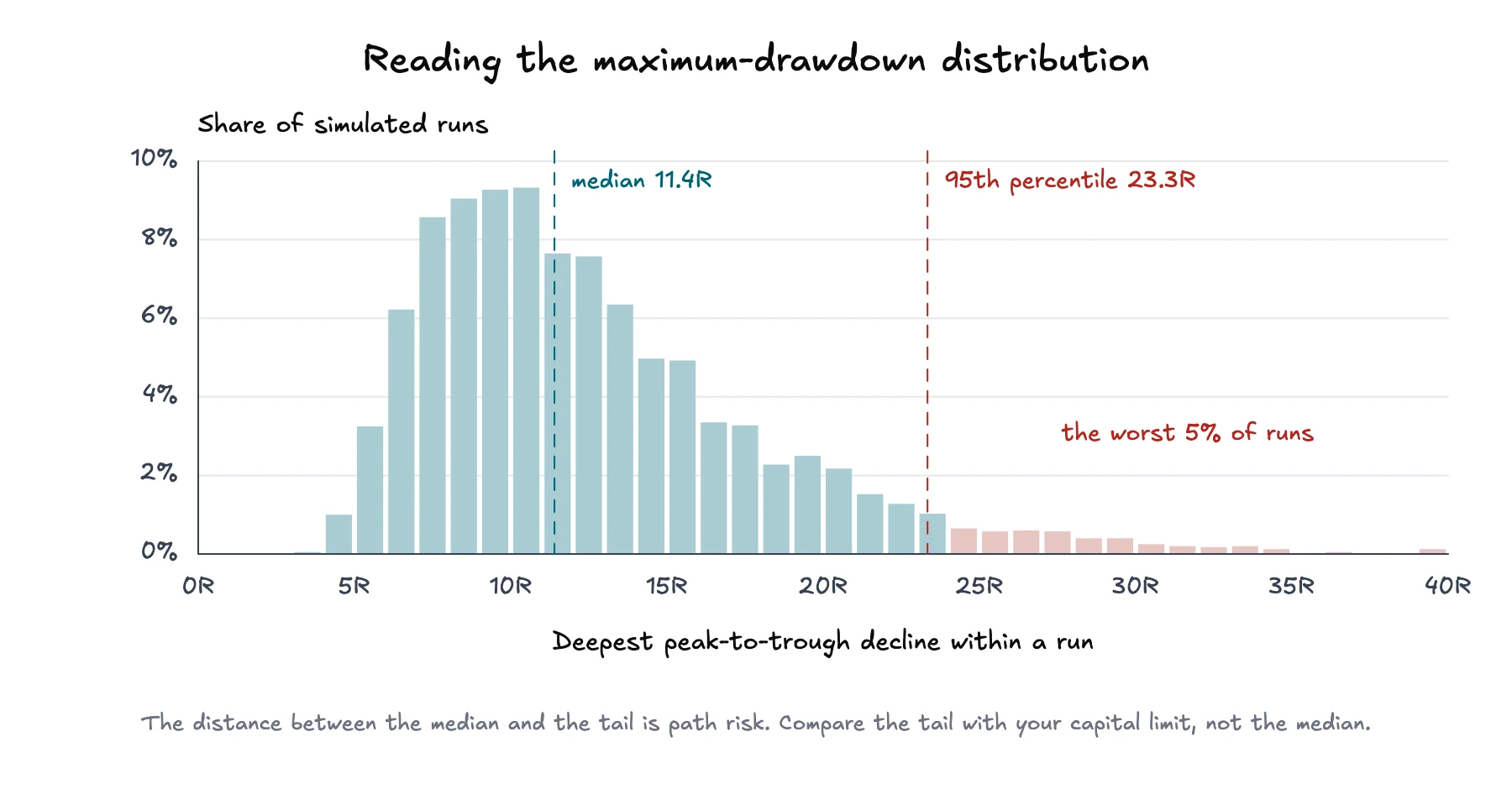
Fan chart cumulative outcomes दिखाता है। Drawdown distribution अलग सवाल का जवाब देता है: हर simulated path अपनी पिछली peak से recovery या अंत तक कितनी नीचे गिरा?
हर run के लिए simulation उस path की maximum peak-to-trough गिरावट record करता है। फिर distribution उन maximum Drawdowns को group करता है। उसका center आम simulated worst decline बताता है और upper tail उन गहरी गिरावटों को दिखाता है जो कम runs में हुईं।
समान runs, अलग सवाल। Median worst decline 11.4R है। हर 20 में से एक run 23.3R से आगे गया।
केवल average नहीं, खास तौर पर tail देखें। सहने योग्य median Drawdown के साथ बहुत बड़ा 95th-percentile Drawdown भी हो सकता है। यह अंतर path risk की जानकारी है। इसकी तुलना अपनी capital constraints और उस point से करें जहां strategy को plan के मुताबिक execute करना संभव नहीं रहेगा।
यह risk of ruin से जुड़ा है, लेकिन समान नहीं है। Drawdown path में peak-to-trough loss मापता है। Ruin के लिए defined capital threshold चाहिए और यह पूछता है कि simulated path कितनी बार उस threshold तक पहुंचा। अगर आप manually set किए win rate, payoff, Trade risk और capital assumptions जांचना चाहते हैं, तो risk-of-ruin simulator उपयोगी है। Monte Carlo analysis आपकी filtered imported Trade history का distribution इस्तेमाल करता है।
Simulation को single Score के बजाय comparison tool की तरह इस्तेमाल करें।
उस strategy या decision से मेल खाता account scope और filters चुनें जिसकी आप review कर रहे हैं।
Output पढ़ने से पहले sample जांचें। Confirm करें कि exclusions, missing values और matching Trades की संख्या स्वीकार्य हैं।
Total performance को ordering luck से अलग करने के लिए पहले reshuffle mode चलाएं।
Median final outcome से पहले maximum-Drawdown tail और losing-streak range पढ़ें।
Projection mode पर जाएं, decision period से मेल खाता horizon चुनें और देखें कि fan कितनी तेजी से चौड़ा होता है।
एक बार में एक ऐसा filter बदलें जिसका कारण साफ हो। Market regime, Setup या account हटाने पर distribution तेजी से बदले, तो पसंद का result चुनने के बजाय कारण जांचें।
Simulation बता सकता है कि observed results sampling और order के प्रति कितने sensitive हैं। यह strategy के Edge को validate नहीं कर सकता, biased input data को ठीक नहीं कर सकता और position size नहीं चुन सकता। Position sizing अलग decision है। Kelly criterion मजबूत assumptions के तहत growth-optimal fraction बताता है, जबकि risk-of-ruin analysis capital threshold पार करने की संभावना पर focus करता है।
Monte Carlo result ऐसे statements को support करता है जो उसके inputs पर conditional हों: इस filtered sample, इस mode, इस horizon और runs की इस संख्या के तहत यह range दिखी। यह future return या Drawdown की guarantee, outcomes की independence या filtered sample के आगे भी representative रहने के दावे को support नहीं करता।
इस limitation के कारण analysis को छोड़ना नहीं चाहिए। इसी कारण source label करना, tails देखना और underlying Trade set बदलने पर test फिर चलाना जरूरी है। इसका value ज्यादा आकर्षक इक्विटी कर्व नहीं है। यह दिखाता है कि समान Trade evidence में पहले से कितनी uncertainty है।